Tutorial 2: Toy Systems

In this tutorial, we will be performing a SEEKR2 calculation on a “Toy System”, that is - a system with one or few particle(s) that move on a relatively simple potential energy surface.

Toy systems can be very useful to benchmark the accuracy of a new method, to improve conceptual understanding of the interaction between a method and a real molecular system, or as a teaching tool about a method.

In this tutorial, we will be using the Entropy Barrier and Muller Potential toy systems.

The Entropy Barrier toy system

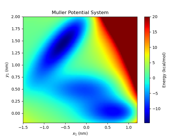
The Muller Potential toy system

Entropy Barrier Toy System

First, to prepare and run the toy systems, it will be helpful to have a sample input XML.

Move to your home directory or other convenient location and clone the seekr2_systems repository.:

cd
git clone https://github.com/seekrcentral/seekr2_systems.git

A number of useful input files can be found in this repository, but we are going to use the input files in the seekr2_systems/systems/toy_systems/ directory. Let’s start by looking at the Entropy Barrier system input.:

cd seekr2_systems/systems/toy_systems

Using Gedit, Vim, or another editor, open up the file “input_entropy_barrier.xml”.

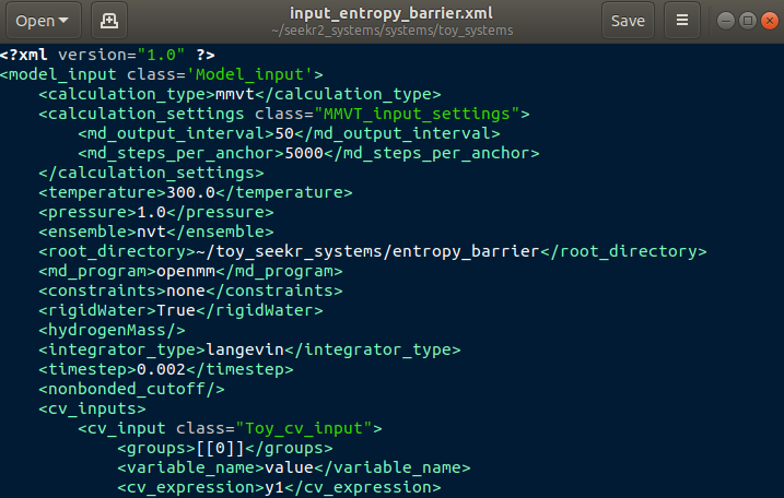
Model input file of the Entropy Barrier toy system.

As with the host/guest system, this input file contains all the information to prepare a SEEKR calculation. Detailed information for all inputs can be found in Model Input Files and some should be familiar from Tutorial 1, but I’m going to highlight a few key changes unique to toy systems.

First, toy systems require their own kind of collective variable (CV). Notice that the CV is of a “Toy_cv_input” type, and its anchors are of the “Toy_cv_anchor” type. Notice that, for a toy system, none of the input require any files except the Model Input File, which is an advantage to running toy systems, as opposed to real molecular systems which need starting coordinate files as well as parameter and topology files.

<groups>

The value “[[0]]” is a Python list of a list, both dimensions of length 1, and this entry indicates that this CV only keeps track of a single group, formed of a single atom, and that’s atom index 0. Toy systems can have any number of atoms, and Toy CVs can keep track of any of those atoms as needed.

<variable_name>

One may change the string representation of the CV’s variable by changing this string. The string “value” should suffice in most any circumstance, although some CVs use the string “radius” to represent their variables.

<cv_expression>

This expression is used to determine anchor location, as well as to construct the mathematical milestone expression. In essence, milestones are constructed along the surfaces where this expression is constant (isosurfaces). In this case, the milestones are constructed where the y-coordinate of the first (and only) atom is constant. (OpenMM expressions start indexing at 1, not 0).

Within the input_anchor objects:

<starting_positions>

Instead of providing a PDB file as starting positions, for a toy system, we provide starting coordinates for each of the particles. This input is a triple-nested list. The outermost layer are “frames” of a toy simulation, in order to use or test the “swarm” capabilities of MMVT. The next layer are the particles in a frame of the swarm. Since this toy system has only one particle, there is only one item in this list. The final layer are the x,y,z coordinates of the particle. Notice that in the first input anchor, there are two frames, making a swarm of size two. In contrast the second anchor has only a single frame. These are in units of nanometers.

At the very end of the Model Input file, one can find the <toy_settings_input> tag. Inside are a number of other settings for the toy system.

<potential_energy_expression>

Define the function of particle positions that describe the potential energy surface.

<num_particles>

The total number of particles in this toy system.

<masses>

A list of masses by particle (in units of AMU).

Create the correct output directory and we are ready to run prepare.py on the model input file, run, and analyze.:

mkdir ~/toy_seekr_systems
cd seekr2/seekr2
python prepare.py input_entropy_barrier.xml.xml
python run.py any ~/toy_seekr_systems/entropy_barrier/model.xml
python converge.py ~/toy_seekr_systems/entropy_barrier/model.xml > converge.txt
python analyze.py ~/toy_seekr_systems/entropy_barrier/model.xml > analyze.txt

All of these commands should work the same for the toy system as they did for the molecular host/guest system. View converge.txt and analyze.txt in Gedit, Vim, or another text file viewer/editor.

One final step involves visualizing the trajectories in the toy system. The seekr2_systems repository contains some scripts for visualizing the results of the toy systems.:

cd ~/seekr2_systems/systems/toy_systems
python entropy_barrier_plot.py

A video should appear that shows the trajectories moving around the Voronoi cells of the Entropy Barrier system. At the bottom of the entropy_barrier_plot.py script, there are some commented lines that will generate a movie that can be played.

Entropy Barrier MMVT trajectories

Muller Potential Toy System

Let us perform the same calculation using the Muller potential.

The model input file for the Muller potential can be found in seekr2_systems/systems/toy_systems. Using Vim, Gedit, or another text editor, open the file “input_muller_potential.xml”. There are a few key differences between the Muller potential and the Entropy Barrier system.

In the <cv_inputs> tag:

<cv_expression>

Now, the <cv_expression> tag has been given a new function: “1.0*y1 - 0.66*x1”. This will cause the milestones to be “slanted” in the coordinate system, unlike the horizontal lines milestones of the Entropy Barrier system.

<openmm_expression>

One may optionally provide the expression that will be used by OpenMM to construct the milestone surfaces, though this is optional.

In the <toy_settings_input> tag:

<potential_energy_expression>

A new expression is needed to use the Muller potential energy landscape.

We will perform the same steps as before.:

cd seekr2/seekr2
python prepare.py input_muller_potential.xml.xml
python run.py any ~/toy_seekr_systems/muller_potential/model.xml
python converge.py ~/toy_seekr_systems/muller_potential/model.xml > converge.txt
python analyze.py ~/toy_seekr_systems/muller_potential/model.xml > analyze.txt

Feel free to examine analyze.txt or converge.txt. One may also make a video of the MMVT simulations in the Muller potential by using the muller_potential_plot.py program.:

cd ~/seekr2_systems/systems/toy_systems
python muller_potential_plot.py

Muller Potential MMVT trajectories